AI with Python – Unsupervised Learning: Clustering

Unsupervised machine learning algorithms do not have any supervisor to provide any sort of guidance. That is why they are closely aligned with what some call true artificial intelligence.

In unsupervised learning, there would be no correct answer and no teacher for the guidance. Algorithms need to discover the interesting pattern in data for learning.

What is Clustering?

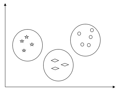
Basically, it is a type of unsupervised learning method and a common technique for statistical data analysis used in many fields. Clustering mainly is a task of dividing the set of observations into subsets, called clusters, in such a way that observations in the same cluster are similar in one sense and they are dissimilar to the observations in other clusters. In simple words, we can say that the main goal of clustering is to group the data on the basis of similarity and dissimilarity.

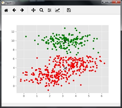
For example, the following diagram shows similar kind of data in different clusters −

Algorithms for Clustering the Data

Following are a few common algorithms for clustering the data −

K-Means algorithm

K-means clustering algorithm is one of the well-known algorithms for clustering the data. We need to assume that the numbers of clusters are already known. This is also called flat clustering. It is an iterative clustering algorithm. The steps given below need to be followed for this algorithm −

Step 1 − We need to specify the desired number of K subgroups.

Step 2 − Fix the number of clusters and randomly assign each data point to a cluster. Or in other words we need to classify our data based on the number of clusters.

In this step, cluster centroids should be computed.

As this is an iterative algorithm, we need to update the locations of K centroids with every iteration until we find the global optima or in other words the centroids reach at their optimal locations.

The following code will help in implementing K-means clustering algorithm in Python. We are going to use the Scikit-learn module.

Let us import the necessary packages −

import matplotlib.pyplot as plt
import seaborn as sns; sns.set()
import numpy as np
from sklearn.cluster import KMeans

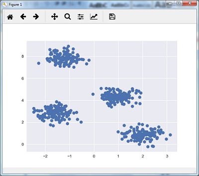
The following line of code will help in generating the two-dimensional dataset, containing four blobs, by using make_blob from the sklearn.dataset package.

from sklearn.datasets.samples_generator import make_blobs

X, y_true = make_blobs(n_samples = 500, centers = 4,
            cluster_std = 0.40, random_state = 0)

We can visualize the dataset by using the following code −

plt.scatter(X[:, 0], X[:, 1], s = 50);
plt.show()

Here, we are initializing kmeans to be the KMeans algorithm, with the required parameter of how many clusters (n_clusters).

kmeans = KMeans(n_clusters = 4)

We need to train the K-means model with the input data.

kmeans.fit(X)
y_kmeans = kmeans.predict(X)
plt.scatter(X[:, 0], X[:, 1], c = y_kmeans, s = 50, cmap = 'viridis')

centers = kmeans.cluster_centers_

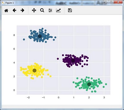
The code given below will help us plot and visualize the machine’s findings based on our data, and the fitment according to the number of clusters that are to be found.

plt.scatter(centers[:, 0], centers[:, 1], c = 'black', s = 200, alpha = 0.5);
plt.show()

Mean Shift Algorithm

It is another popular and powerful clustering algorithm used in unsupervised learning. It does not make any assumptions hence it is a non-parametric algorithm. It is also called hierarchical clustering or mean shift cluster analysis. Followings would be the basic steps of this algorithm −

• First of all, we need to start with the data points assigned to a cluster of their own.

• Now, it computes the centroids and update the location of new centroids.

• By repeating this process, we move closer the peak of cluster i.e. towards the region of higher density.

• This algorithm stops at the stage where centroids do not move anymore.

With the help of following code we are implementing Mean Shift clustering algorithm in Python. We are going to use Scikit-learn module.

Let us import the necessary packages −

import numpy as np
from sklearn.cluster import MeanShift
import matplotlib.pyplot as plt
from matplotlib import style
style.use("ggplot")

The following code will help in generating the two-dimensional dataset, containing four blobs, by using make_blob from the sklearn.dataset package.

from sklearn.datasets.samples_generator import make_blobs

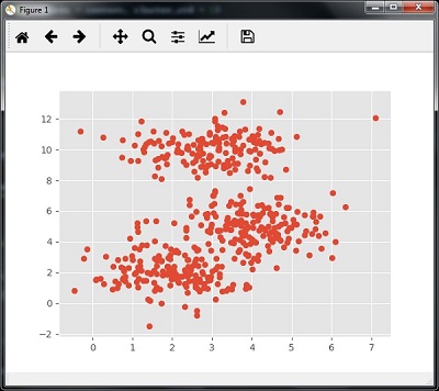
We can visualize the dataset with the following code

centers = [[2,2],[4,5],[3,10]]
X, _ = make_blobs(n_samples = 500, centers = centers, cluster_std = 1)
plt.scatter(X[:,0],X[:,1])
plt.show()

Now, we need to train the Mean Shift cluster model with the input data.

ms = MeanShift()
ms.fit(X)
labels = ms.labels_
cluster_centers = ms.cluster_centers_

The following code will print the cluster centers and the expected number of cluster as per the input data −

print(cluster_centers)
n_clusters_ = len(np.unique(labels))
print("Estimated clusters:", n_clusters_)
[[ 3.23005036 3.84771893]
[ 3.02057451 9.88928991]]
Estimated clusters: 2

The code given below will help plot and visualize the machine’s findings based on our data, and the fitment according to the number of clusters that are to be found.

colors = 10*['r.','g.','b.','c.','k.','y.','m.']
   for i in range(len(X)):
   plt.plot(X[i][0], X[i][1], colors[labels[i]], markersize = 10)
plt.scatter(cluster_centers[:,0],cluster_centers[:,1],
   marker = "x",color = 'k', s = 150, linewidths = 5, zorder = 10)
plt.show()

Measuring the Clustering Performance

The real world data is not naturally organized into number of distinctive clusters. Due to this reason, it is not easy to visualize and draw inferences. That is why we need to measure the clustering performance as well as its quality. It can be done with the help of silhouette analysis.

Silhouette Analysis

This method can be used to check the quality of clustering by measuring the distance between the clusters. Basically, it provides a way to assess the parameters like number of clusters by giving a silhouette score. This score is a metric that measures how close each point in one cluster is to the points in the neighboring clusters.

Analysis of silhouette score

The score has a range of [-1, 1]. Following is the analysis of this score −

• Score of +1 − Score near +1 indicates that the sample is far away from the neighboring cluster.

• Score of 0 − Score 0 indicates that the sample is on or very close to the decision boundary between two neighboring clusters.

• Score of -1 − Negative score indicates that the samples have been assigned to the wrong clusters.

Calculating Silhouette Score

In this section, we will learn how to calculate the silhouette score.

Silhouette score can be calculated by using the following formula −

$$silhouette score = \frac{\left ( p-q \right )}{max\left ( p,q \right )}$$

Here, 𝑝 is the mean distance to the points in the nearest cluster that the data point is not a part of. And, 𝑞 is the mean intra-cluster distance to all the points in its own cluster.

For finding the optimal number of clusters, we need to run the clustering algorithm again by importing the metrics module from the sklearn package. In the following example, we will run the K-means clustering algorithm to find the optimal number of clusters −

Import the necessary packages as shown −

import matplotlib.pyplot as plt
import seaborn as sns; sns.set()
import numpy as np
from sklearn.cluster import KMeans

With the help of the following code, we will generate the two-dimensional dataset, containing four blobs, by using make_blob from the sklearn.dataset package.

from sklearn.datasets.samples_generator import make_blobs

X, y_true = make_blobs(n_samples = 500, centers = 4, cluster_std = 0.40, random_state = 0)

Initialize the variables as shown −

scores = []
values = np.arange(2, 10)

We need to iterate the K-means model through all the values and also need to train it with the input data.

for num_clusters in values:
kmeans = KMeans(init = 'k-means++', n_clusters = num_clusters, n_init = 10)
kmeans.fit(X)

Now, estimate the silhouette score for the current clustering model using the Euclidean distance metric −

score = metrics.silhouette_score(X, kmeans.labels_,
metric = 'euclidean', sample_size = len(X))

The following line of code will help in displaying the number of clusters as well as Silhouette score.

print("\nNumber of clusters =", num_clusters)
print("Silhouette score =", score)
scores.append(score)

You will receive the following output −

>Number of clusters = 9
Silhouette score = 0.340391138371

num_clusters = np.argmax(scores) + values[0]
print('\nOptimal number of clusters =', num_clusters)

Now, the output for optimal number of clusters would be as follows −

>Optimal number of clusters = 2

Finding Nearest Neighbors

If we want to build recommender systems such as a movie recommender system then we need to understand the concept of finding the nearest neighbors. It is because the recommender system utilizes the concept of nearest neighbors.

The concept of finding nearest neighbors may be defined as the process of finding the closest point to the input point from the given dataset. The main use of this KNN)K-nearest neighbors) algorithm is to build classification systems that classify a data point on the proximity of the input data point to various classes.

The Python code given below helps in finding the K-nearest neighbors of a given data set −

Import the necessary packages as shown below. Here, we are using the NearestNeighbors module from the sklearn package

import numpy as np
import matplotlib.pyplot as plt
from sklearn.neighbors import NearestNeighbors

Let us now define the input data −

A = np.array([[3.1, 2.3], [2.3, 4.2], [3.9, 3.5], [3.7, 6.4], [4.8, 1.9], 
             [8.3, 3.1], [5.2, 7.5], [4.8, 4.7], [3.5, 5.1], [4.4, 2.9],])

Now, we need to define the nearest neighbors −

k = 3

We also need to give the test data from which the nearest neighbors is to be found −

test_data = [3.3, 2.9]

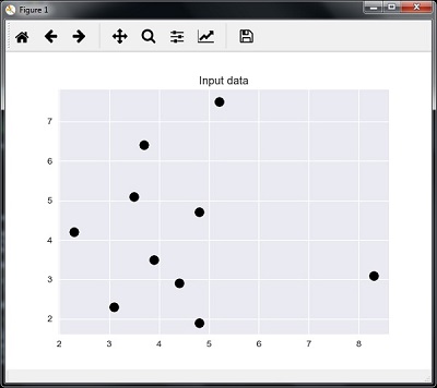
The following code can visualize and plot the input data defined by us −

plt.figure()
plt.title('Input data')
plt.scatter(A[:,0], A[:,1], marker = 'o', s = 100, color = 'black')

Now, we need to build the K Nearest Neighbor. The object also needs to be trained

knn_model = NearestNeighbors(n_neighbors = k, algorithm = 'auto').fit(X)
distances, indices = knn_model.kneighbors([test_data])

Now, we can print the K nearest neighbors as follows

print("\nK Nearest Neighbors:")
for rank, index in enumerate(indices[0][:k], start = 1):
   print(str(rank) + " is", A[index])

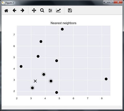
We can visualize the nearest neighbors along with the test data point

plt.figure()
plt.title('Nearest neighbors')
plt.scatter(A[:, 0], X[:, 1], marker = 'o', s = 100, color = 'k')
plt.scatter(A[indices][0][:][:, 0], A[indices][0][:][:, 1],
   marker = 'o', s = 250, color = 'k', facecolors = 'none')
plt.scatter(test_data[0], test_data[1],
   marker = 'x', s = 100, color = 'k')
plt.show()

Output

K Nearest Neighbors

>1 is [ 3.1 2.3]
2 is [ 3.9 3.5]
3 is [ 4.4 2.9]

K-Nearest Neighbors Classifier

A K-Nearest Neighbors (KNN) classifier is a classification model that uses the nearest neighbors algorithm to classify a given data point. We have implemented the KNN algorithm in the last section, now we are going to build a KNN classifier using that algorithm.

Concept of KNN Classifier

The basic concept of K-nearest neighbor classification is to find a predefined number, i.e., the ‘k’ – of training samples closest in distance to a new sample, which has to be classified. New samples will get their label from the neighbors itself. The KNN classifiers have a fixed user defined constant for the number of neighbors which have to be determined. For the distance, standard Euclidean distance is the most common choice. The KNN Classifier works directly on the learned samples rather than creating the rules for learning. The KNN algorithm is among the simplest of all machine learning algorithms. It has been quite successful in a large number of classification and regression problems, for example, character recognition or image analysis.

Example

We are building a KNN classifier to recognize digits. For this, we will use the MNIST dataset. We will write this code in the Jupyter Notebook.

Import the necessary packages as shown below.

Here we are using the KNeighborsClassifier module from the sklearn.neighbors package −

from sklearn.datasets import *
import pandas as pd
%matplotlib inline
from sklearn.neighbors import KNeighborsClassifier
import matplotlib.pyplot as plt
import numpy as np

The following code will display the image of digit to verify what image we have to test −

def Image_display(i):
   plt.imshow(digit['images'][i],cmap = 'Greys_r')
   plt.show()

Now, we need to load the MNIST dataset. Actually there are total 1797 images but we are using the first 1600 images as training sample and the remaining 197 would be kept for testing purpose.

digit = load_digits()
digit_d = pd.DataFrame(digit['data'][0:1600])

Now, on displaying the images we can see the output as follows −

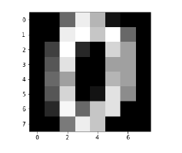
>Image_display(0)

Image_display(0)

Image of 0 is displayed as follows −

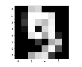
Image_display(9)

Image of 9 is displayed as follows −

digit.keys()

Now, we need to create the training and testing data set and supply testing data set to the KNN classifiers.

train_x = digit['data'][:1600]
train_y = digit['target'][:1600]
KNN = KNeighborsClassifier(20)
KNN.fit(train_x,train_y)

The following output will create the K nearest neighbor classifier constructor −

>KNeighborsClassifier(algorithm = 'auto', leaf_size = 30, metric = 'minkowski',
   metric_params = None, n_jobs = 1, n_neighbors = 20, p = 2,
   weights = 'uniform')

We need to create the testing sample by providing any arbitrary number greater than 1600, which were the training samples.

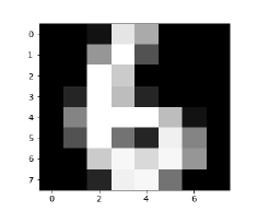
test = np.array(digit['data'][1725])
test1 = test.reshape(1,-1)
Image_display(1725)

Image_display(6)

Image of 6 is displayed as follows −

Now we will predict the test data as follows −

KNN.predict(test1)

The above code will generate the following output −

>array([6])

Now, consider the following −

digit['target_names']

The above code will generate the following output −

>array([0, 1, 2, 3, 4, 5, 6, 7, 8, 9])