AI with Python – Supervised Learning: Regression

Regression is one of the most important statistical and machine learning tools. We would not be wrong to say that the journey of machine learning starts from regression. It may be defined as the parametric technique that allows us to make decisions based upon data or in other words allows us to make predictions based upon data by learning the relationship between input and output variables. Here, the output variables dependent on the input variables, are continuous-valued real numbers. In regression, the relationship between input and output variables matters and it helps us in understanding how the value of the output variable changes with the change of input variable. Regression is frequently used for prediction of prices, economics, variations, and so on.

Building Regressors in Python

In this section, we will learn how to build single as well as multivariable regressor.

Linear Regressor/Single Variable Regressor

Let us important a few required packages −

import numpy as np
from sklearn import linear_model
import sklearn.metrics as sm
import matplotlib.pyplot as plt

Now, we need to provide the input data and we have saved our data in the file named linear.txt.

input = 'D:/ProgramData/linear.txt'

We need to load this data by using the np.loadtxt function.

input_data = np.loadtxt(input, delimiter=',')
X, y = input_data[:, :-1], input_data[:, -1]

The next step would be to train the model. Let us give training and testing samples.

training_samples = int(0.6 * len(X))
testing_samples = len(X) - num_training

X_train, y_train = X[:training_samples], y[:training_samples]

X_test, y_test = X[training_samples:], y[training_samples:]

Now, we need to create a linear regressor object.

reg_linear = linear_model.LinearRegression()

Train the object with the training samples.

reg_linear.fit(X_train, y_train)

We need to do the prediction with the testing data.

y_test_pred = reg_linear.predict(X_test)

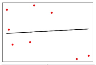
Now plot and visualize the data.

plt.scatter(X_test, y_test, color = 'red')
plt.plot(X_test, y_test_pred, color = 'black', linewidth = 2)
plt.xticks(())
plt.yticks(())
plt.show()

Output

Now, we can compute the performance of our linear regression as follows −

print("Performance of Linear regressor:")
print("Mean absolute error =", round(sm.mean_absolute_error(y_test, y_test_pred), 2))
print("Mean squared error =", round(sm.mean_squared_error(y_test, y_test_pred), 2))
print("Median absolute error =", round(sm.median_absolute_error(y_test, y_test_pred), 2))
print("Explain variance score =", round(sm.explained_variance_score(y_test, y_test_pred),
2))
print("R2 score =", round(sm.r2_score(y_test, y_test_pred), 2))

Output

Performance of Linear Regressor −

>Mean absolute error = 1.78
Mean squared error = 3.89
Median absolute error = 2.01
Explain variance score = -0.09
R2 score = -0.09

In the above code, we have used this small data. If you want some big dataset then you can use sklearn.dataset to import bigger dataset.

2,4.82.9,4.72.5,53.2,5.56,57.6,43.2,0.92.9,1.92.4,
3.50.5,3.41,40.9,5.91.2,2.583.2,5.65.1,1.54.5,
1.22.3,6.32.1,2.8

Multivariable Regressor

First, let us import a few required packages −

import numpy as np
from sklearn import linear_model
import sklearn.metrics as sm
import matplotlib.pyplot as plt
from sklearn.preprocessing import PolynomialFeatures

Now, we need to provide the input data and we have saved our data in the file named linear.txt.

input = 'D:/ProgramData/Mul_linear.txt'

We will load this data by using the np.loadtxt function.

input_data = np.loadtxt(input, delimiter=',')
X, y = input_data[:, :-1], input_data[:, -1]

The next step would be to train the model; we will give training and testing samples.

training_samples = int(0.6 * len(X))
testing_samples = len(X) - num_training

X_train, y_train = X[:training_samples], y[:training_samples]

X_test, y_test = X[training_samples:], y[training_samples:]

Now, we need to create a linear regressor object.

reg_linear_mul = linear_model.LinearRegression()

Train the object with the training samples.

reg_linear_mul.fit(X_train, y_train)

Now, at last we need to do the prediction with the testing data.

>y_test_pred = reg_linear_mul.predict(X_test)

print("Performance of Linear regressor:")
print("Mean absolute error =", round(sm.mean_absolute_error(y_test, y_test_pred), 2))
print("Mean squared error =", round(sm.mean_squared_error(y_test, y_test_pred), 2))
print("Median absolute error =", round(sm.median_absolute_error(y_test, y_test_pred), 2))
print("Explain variance score =", round(sm.explained_variance_score(y_test, y_test_pred), 2))
print("R2 score =", round(sm.r2_score(y_test, y_test_pred), 2))

Output

Performance of Linear Regressor −

>Mean absolute error = 0.6
Mean squared error = 0.65
Median absolute error = 0.41
Explain variance score = 0.34
R2 score = 0.33

Now, we will create a polynomial of degree 10 and train the regressor. We will provide the sample data point.

polynomial = PolynomialFeatures(degree = 10)
X_train_transformed = polynomial.fit_transform(X_train)
datapoint = [[2.23, 1.35, 1.12]]
poly_datapoint = polynomial.fit_transform(datapoint)

poly_linear_model = linear_model.LinearRegression()
poly_linear_model.fit(X_train_transformed, y_train)
print("\nLinear regression:\n", reg_linear_mul.predict(datapoint))
print("\nPolynomial regression:\n", poly_linear_model.predict(poly_datapoint))

Output

Linear regression −

>[2.40170462]

Polynomial regression −

>[1.8697225]

In the above code, we have used this small data. If you want a big dataset then, you can use sklearn.dataset to import a bigger dataset.

2,4.8,1.2,3.22.9,4.7,1.5,3.62.5,5,2.8,23.2,5.5,3.5,2.16,5,
2,3.27.6,4,1.2,3.23.2,0.9,2.3,1.42.9,1.9,2.3,1.22.4,3.5,
2.8,3.60.5,3.4,1.8,2.91,4,3,2.50.9,5.9,5.6,0.81.2,2.58,
3.45,1.233.2,5.6,2,3.25.1,1.5,1.2,1.34.5,1.2,4.1,2.32.3,
6.3,2.5,3.22.1,2.8,1.2,3.6