

The Knight’s tour problem
The Knight’s tour problem
Backtracking is an algorithmic paradigm that tries different solutions until finds a solution that “works”. Problems which are typically solved using backtracking technique have the following property in common. These problems can only be solved by trying every possible configuration and each configuration is tried only once. A Naive solution for these problems is to try all configurations and output a configuration that follows given problem constraints. Backtracking works in an incremental way and is an optimization over the Naive solution where all possible configurations are generated and tried.
For example, consider the following Knight’s Tour problem.
The knight is placed on the first block of an empty board and, moving according to the rules of chess, must visit each square exactly once.
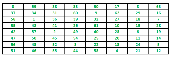
Path followed by Knight to cover all the cells
Following is chessboard with 8 x 8 cells. Numbers in cells indicate move number of Knight.
Let us first discuss the Naive algorithm for this problem and then the Backtracking algorithm.
Naive Algorithm for Knight’s tour
The Naive Algorithm is to generate all tours one by one and check if the generated tour satisfies the constraints.
while there are untried tours
{
   generate the next tour
   if this tour covers all squares
   {
      print this path;
   }
}
Backtracking works in an incremental way to attack problems. Typically, we start from an empty solution vector and one by one add items (Meaning of item varies from problem to problem. In context of Knight’s tour problem, an item is a Knight’s move). When we add an item, we check if adding the current item violates the problem constraint, if it does then we remove the item and try other alternatives. If none of the alternatives work out then we go to the previous stage and remove the item added in the previous stage. If we reach the initial stage back then we say that no solution exists. If adding an item doesn’t violate constraints then we recursively add items one by one. If the solution vector becomes complete then we print the solution.
Backtracking Algorithm for Knight’s tour
Following is the Backtracking algorithm for Knight’s tour problem.
If all squares are visited
    print the solution
Else
   a) Add one of the next moves to solution vector and recursively
   check if this move leads to a solution. (A Knight can make maximum
   eight moves. We choose one of the 8 moves in this step).
   b) If the move chosen in the above step doesn't lead to a solution
   then remove this move from the solution vector and try other
   alternative moves.
   c) If none of the alternatives work then return false (Returning false
   will remove the previously added item in recursion and if false is
   returned by the initial call of recursion then "no solution exists" )
Following are implementations for Knight’s tour problem. It prints one of the possible solutions in 2D matrix form. Basically, the output is a 2D 8*8 matrix with numbers from 0 to 63 and these numbers show steps made by Knight.
C
// C program for Knight Tour problem
#include<stdio.h>
#define N 8

int solveKTUtil(int x, int y, int movei, int sol[N][N],
                int xMove[],  int yMove[]);

/* A utility function to check if i,j are valid indexes
   for N*N chessboard */
bool isSafe(int x, int y, int sol[N][N])
{
    return ( x >= 0 && x < N && y >= 0 &&
             y < N && sol[x][y] == -1);
}

/* A utility function to print solution matrix sol[N][N] */
void printSolution(int sol[N][N])
{
    for (int x = 0; x < N; x++)
    {
        for (int y = 0; y < N; y++)
            printf(" %2d ", sol[x][y]);
        printf("\n");
    }
}

/* This function solves the Knight Tour problem using
   Backtracking.  This function mainly uses solveKTUtil()
   to solve the problem. It returns false if no complete
   tour is possible, otherwise return true and prints the
   tour.
   Please note that there may be more than one solutions,
   this function prints one of the feasible solutions.  */
bool solveKT()
{
    int sol[N][N];

    /* Initialization of solution matrix */
    for (int x = 0; x < N; x++)
        for (int y = 0; y < N; y++)
            sol[x][y] = -1;

    /* xMove[] and yMove[] define next move of Knight.
       xMove[] is for next value of x coordinate
       yMove[] is for next value of y coordinate */
    int xMove[8] = {  2, 1, -1, -2, -2, -1,  1,  2 };
    int yMove[8] = {  1, 2,  2,  1, -1, -2, -2, -1 };

    // Since the Knight is initially at the first block
    sol[0][0]  = 0;

    /* Start from 0,0 and explore all tours using
       solveKTUtil() */
    if (solveKTUtil(0, 0, 1, sol, xMove, yMove) == false)
    {
        printf("Solution does not exist");
        return false;
    }
    else
        printSolution(sol);

    return true;
}

/* A recursive utility function to solve Knight Tour
   problem */
int solveKTUtil(int x, int y, int movei, int sol[N][N],
                int xMove[N], int yMove[N])
{
   int k, next_x, next_y;
   if (movei == N*N)
       return true;

   /* Try all next moves from the current coordinate x, y */
   for (k = 0; k < 8; k++)
   {
       next_x = x + xMove[k];
       next_y = y + yMove[k];
       if (isSafe(next_x, next_y, sol))
       {
         sol[next_x][next_y] = movei;
         if (solveKTUtil(next_x, next_y, movei+1, sol,
                         xMove, yMove) == true)
             return true;
         else
             sol[next_x][next_y] = -1;// backtracking
       }
   }

   return false;
}

/* Driver program to test above functions */
int main()
{
    solveKT();
    return 0;
}
Java
// Java program for Knight Tour problem
class KnightTour {
    static int N = 8;

    /* A utility function to check if i,j are
       valid indexes for N*N chessboard */
    static boolean isSafe(int x, int y, int sol[][]) {
        return (x >= 0 && x < N && y >= 0 &&
                y < N && sol[x][y] == -1);
    }

    /* A utility function to print solution
       matrix sol[N][N] */
    static void printSolution(int sol[][]) {
        for (int x = 0; x < N; x++) {
            for (int y = 0; y < N; y++)
                System.out.print(sol[x][y] + " ");
            System.out.println();
        }
    }

    /* This function solves the Knight Tour problem
       using Backtracking.  This  function mainly
       uses solveKTUtil() to solve the problem. It
       returns false if no complete tour is possible,
       otherwise return true and prints the tour.
       Please note that there may be more than one
       solutions, this function prints one of the
       feasible solutions.  */
    static boolean solveKT() {
        int sol[][] = new int[8][8];

        /* Initialization of solution matrix */
        for (int x = 0; x < N; x++)
            for (int y = 0; y < N; y++)
                sol[x][y] = -1;

       /* xMove[] and yMove[] define next move of Knight.
          xMove[] is for next value of x coordinate
          yMove[] is for next value of y coordinate */
        int xMove[] = {2, 1, -1, -2, -2, -1, 1, 2};
        int yMove[] = {1, 2, 2, 1, -1, -2, -2, -1};

        // Since the Knight is initially at the first block
        sol[0][0] = 0;

        /* Start from 0,0 and explore all tours using
           solveKTUtil() */
        if (!solveKTUtil(0, 0, 1, sol, xMove, yMove)) {
            System.out.println("Solution does not exist");
            return false;
        } else
            printSolution(sol);

        return true;
    }

    /* A recursive utility function to solve Knight
       Tour problem */
    static boolean solveKTUtil(int x, int y, int movei,
                               int sol[][], int xMove[],
                               int yMove[]) {
        int k, next_x, next_y;
        if (movei == N * N)
            return true;

        /* Try all next moves from the current coordinate
            x, y */
        for (k = 0; k < 8; k++) {
            next_x = x + xMove[k];
            next_y = y + yMove[k];
            if (isSafe(next_x, next_y, sol)) {
                sol[next_x][next_y] = movei;
                if (solveKTUtil(next_x, next_y, movei + 1,
                                sol, xMove, yMove))
                    return true;
                else
                    sol[next_x][next_y] = -1;// backtracking
            }
        }

        return false;
    }

    /* Driver program to test above functions */
    public static void main(String args[]) {
        solveKT();
    }
}
// This code is contributed by Abhishek Shankhadhar
C#
// C# program for
// Knight Tour problem
using System;

class GFG
{
    static int N = 8;

    /* A utility function to
    check if i,j are valid
    indexes for N*N chessboard */
    static bool isSafe(int x, int y,
                       int[,] sol)
    {
        return (x >= 0 && x < N &&
                y >= 0 && y < N &&
                sol[x, y] == -1);
    }

    /* A utility function to
    print solution matrix sol[N][N] */
    static void printSolution(int[,] sol)
    {
        for (int x = 0; x < N; x++)
        {
            for (int y = 0; y < N; y++)
                Console.Write(sol[x, y] + " ");
            Console.WriteLine();
        }
    }

    /* This function solves the
    Knight Tour problem using
    Backtracking. This function
    mainly uses solveKTUtil() to
    solve the problem. It returns
    false if no complete tour is
    possible, otherwise return true
    and prints the tour. Please note
    that there may be more than one
    solutions, this function prints
    one of the feasible solutions. */
    static bool solveKT()
     {
        int[,] sol = new int[8, 8];

        /* Initialization of
        solution matrix */
        for (int x = 0; x < N; x++)
            for (int y = 0; y < N; y++)
                sol[x, y] = -1;

     /* xMove[] and yMove[] define
        next move of Knight.
        xMove[] is for next
        value of x coordinate
        yMove[] is for next
        value of y coordinate */
        int[] xMove = {2, 1, -1, -2,
                      -2, -1, 1, 2};
        int[] yMove = {1, 2, 2, 1,
                      -1, -2, -2, -1};

        // Since the Knight is
        // initially at the first block
        sol[0, 0] = 0;

        /* Start from 0,0 and explore
        all tours using solveKTUtil() */
        if (!solveKTUtil(0, 0, 1, sol,
                         xMove, yMove))
        {
            Console.WriteLine("Solution does "+
                                  "not exist");
            return false;
        }
        else
            printSolution(sol);

        return true;
    }

    /* A recursive utility function
    to solve Knight Tour problem */
    static bool solveKTUtil(int x, int y, int movei,
                            int[,] sol, int[] xMove,
                            int[] yMove)
    {
        int k, next_x, next_y;
        if (movei == N * N)
            return true;

        /* Try all next moves from
        the current coordinate x, y */
        for (k = 0; k < 8; k++)
        {
            next_x = x + xMove[k];
            next_y = y + yMove[k];
            if (isSafe(next_x, next_y, sol))
            {
                sol[next_x,next_y] = movei;
                if (solveKTUtil(next_x, next_y, movei +
                                 1, sol, xMove, yMove))
                    return true;
                else
                    // backtracking
                    sol[next_x,next_y] = -1;
            }
        }

        return false;
    }

    // Driver Code
    public static void Main()
    {
        solveKT();
    }
}

// This code is contributed by mits.
Output:
  0  59  38  33  30  17   8  63
 37  34  31  60   9  62  29  16
 58   1  36  39  32  27  18   7
 35  48  41  26  61  10  15  28
 42  57   2  49  40  23   6  19
 47  50  45  54  25  20  11  14
 56  43  52   3  22  13  24   5
 51  46  55  44  53   4  21  12
Note that Backtracking is not the best solution for the Knight’s tour problem. See below article for other better solutions. The purpose of this post is to explain Backtracking with an example.
Warnsdorff’s algorithm for Knight’s tour problem
References:
http://see.stanford.edu/materials/icspacs106b/H19-RecBacktrackExamples.pdf
http://www.cis.upenn.edu/~matuszek/cit594-2009/Lectures/35-backtracking.ppt
http://mathworld.wolfram.com/KnightsTour.html
http://en.wikipedia.org/wiki/Knight%27s_tour
Backtracking
A Time Complexity
A Time Complexity Question
What is the time complexity of following function fun()? Assume that log(x) returns log value in base 2.
void fun()
{
   int i, j;
   for (i=1; i<=n; i++)
      for (j=1; j<=log(i); j++)
         printf("GeeksforGeeks");
}
Time Complexity of the above function can be written as Θ(log 1) + Θ(log 2) + Θ(log 3) + . . . . + Θ(log n) which is Θ (log n!)
Order of growth of ‘log n!’ and ‘n log n’ is same for large values of n, i.e., Θ (log n!) = Θ(n log n). So time complexity of fun() is Θ(n log n).
The expression Θ(log n!) = Θ(n log n) can be easily derived from following Stirling’s approximation (or Stirling’s formula).
log n! = n log n - n + O(log(n))
Please write comments if you find anything incorrect, or you want to share more information about the topic discussed above.
Sources:
http://en.wikipedia.org/wiki/Stirling%27s_approximation
Time Complexity of building a heap
Consider the following algorithm for building a Heap of an input array A.
BUILD-HEAP(A)
    heapsize := size(A);
    for i := floor(heapsize/2) downto 1
        do HEAPIFY(A, i);
    end for
END
A quick look over the above algorithm suggests that the running time is  , since each call to Heapify costs
  and Build-Heap makes
  such calls.
This upper bound, though correct, is not asymptotically tight.
We can derive a tighter bound by observing that the running time of Heapify depends on the height of the tree ‘h’ (which is equal to lg(n), where n is number of nodes) and the heights of most sub-trees are small.
The height ’h’ increases as we move upwards along the tree. Line-3 of Build-Heap runs a loop from the index of the last internal node (heapsize/2) with height=1, to the index of root(1) with height = lg(n). Hence, Heapify takes different time for each node, which is  .
.
For finding the Time Complexity of building a heap, we must know the number of nodes having height h.
For this we use the fact that, A heap of size n has at most  nodes with height h.
Now to derive the time complexity, we express the total cost of Build-Heap as-
(1) 
Step 2 uses the properties of the Big-Oh notation to ignore the ceiling function and the constant 2( ). Similarly in Step three, the upper limit of the summation can be increased to infinity since we are using Big-Oh notation.
Sum of infinite G.P. (x < 1)
(2) 
On differentiating both sides and multiplying by x, we get
(3) 
Putting the result obtained in (3) back in our derivation (1), we get
(4) 
Hence Proved that the Time complexity for Building a Binary Heap is .
Reference :
http://www.cs.sfu.ca/CourseCentral/307/petra/2009/SLN_2.pdf
Time Complexity where loop variable is incremented by 1, 2, 3, 4 ..
What is the time complexity of below code?
void fun(int n)
{
   int j = 1, i = 0;
   while (i < n)
   {
       // Some O(1) task
       i = i + j;
       j++;
   }
}
The loop variable ‘i’ is incremented by 1, 2, 3, 4, … until i becomes greater than or equal to n.
The value of i is x(x+1)/2 after x iterations. So if loop runs x times, then x(x+1)/2 < n. Therefore time complexity can be written as Θ(√n).
Time Complexity of Loop with Powers
What is the time complexity of below function?
void fun(int n, int k)
{
    for (int i=1; i<=n; i++)
    {
      int p = pow(i, k);
      for (int j=1; j<=p; j++)
      {
          // Some O(1) work
      }
    }
}
Time complexity of above function can be written as 1k + 2k + 3k + … n1k.
Let us try few examples:
k=1
Sum = 1 + 2 + 3 ... n
    = n(n+1)/2
    = n2 + n/2

k=2
Sum = 12 + 22 + 32 + ... n12.
    = n(n+1)(2n+1)/6
    = n3/3 + n2/2 + n/6

k=3
Sum = 13 + 23 + 33 + ... n13.
    = n2(n+1)2/4
    = n4/4 + n3/2 + n2/4
In general, asymptotic value can be written as (nk+1)/(k+1) + Θ(nk)
Note that, in asymptotic notations like Θ we can always ignore lower order terms. So the time complexity is Θ(nk+1/ (k+1))
Performance of loops (A caching question)
Consider below two C language functions to compute sum of elements in a 2D array. Ignoring the compiler optimizations, which of the two is better implementation of sum?
// Function 1
int fun1(int arr[R][C])
{
    int sum = 0;
    for (int i=0; i<R; i++)
      for (int j=0; j<C; j++)
          sum += arr[i][j];
}

// Function 2
int fun2(int arr[R][C])
{
    int sum = 0;
    for (int j=0; j<C; j++)
      for (int i=0; i<R; i++)
          sum += arr[i][j];
}
In C/C++, elements are stored in Row-Major order. So the first implementation has better spatial locality (nearby memory locations are referenced in successive iterations). Therefore, first implementation should always be preferred for iterating multidimensional arrays.
Polynomial Time Approximation Scheme
Polynomial Time Approximation Scheme
It is a very well know fact that there is no known polynomial time solution for NP-Complete problems and these problems occur a lot in the real world (See this, this and this for example). So there must be a way to handle them. We have seen algorithms to these problems which are p approximate (For example 2 approximate for Travelling Salesman). Can we do better?
Polynomial Time Approximation Scheme (PTAS) is a type of approximate algorithms that provide user to control over accuracy which is a desirable feature. These algorithms take an additional parameter ε > 0 and provide a solution that is (1 + ε) approximate for minimization and (1 – ε) for maximization. For example, consider a minimization problem, if ε is 0.5, then the solution provided by the PTAS algorithm is 1.5 approximate. The running time of PTAS must be polynomial in terms of n, however, it can be exponential in terms of ε.
In PTAS algorithms, the exponent of the polynomial can increase dramatically as ε reduces, for example if the runtime is O(n(1/ε)!) which is a problem. There is a stricter scheme, Fully Polynomial Time Approximation Scheme (FPTAS). In FPTAS, algorithm need to polynomial in both the problem size n and 1/ε.
Example (0-1 knapsack problem):
We know that 0-1 knapsack is NP Complete. There is a DP based pseudo polynomial solution for this. But if input values are high, then the solution becomes infeasible and there is a need of approximate solution. One approximate solution is to use Greedy Approach (compute value per kg for all items and put the highest value per kg first if it is smaller than W), but Greedy approach is not PTAS, so we don’t have control over accuracy.
Below is a FPTAS solution for 0-1 Knapsack problem:
Input:
W (Capacity of Knapsack)
val[0..n-1] (Values of Items)
wt[0..n-1] (Weights of Items)
- Find the maximum valued item, i.e., find maximum value in val[]. Let this maximum value be maxVal.
- Compute adjustment factor k for all values
k = (maxVal * ε) / n
- Adjust all values, i.e., create a new array val'[] that values divided by k. Do following for every value val[i].
val'[i] = floor(val[i] / k)
- Run DP based solution for reduced values, i,e, val'[0..n-1] and all other parameter same.
The above solution works in polynomial time in terms of both n and ε. The solution provided by this FPTAS is (1 – ε) approximate. The idea is to rounds off some of the least significant digits of values then they will be bounded by a polynomial and 1/ε.
Example:
val[] = {12, 16, 4, 8}
wt[]  = {3, 4, 5, 2}
W = 10
ε = 0.5

maxVal = 16 [maximum value in val[]]
Adjustment factor, k = (16 * 0.5)/4 = 2.0

Now we apply DP based solution on below modified
instance of problem.

val'[] = {6, 8, 2, 4}  [ val'[i] = floor(val[i]/k) ]
wt[] = {3, 4, 5, 2}
W = 10
How is the solution (1 – ε) * OPT?
Here OPT is the optimal value. Let S be the set produced by above FPTAS algorithm and total value of S be val(S). We need to show that
val(S) >= (1 - ε)*OPT
Let O be the set produced by optimal solution (the solution with total value OPT), i.e., val(O) = OPT.
       val(O) - k*val'(O) <= n*k
       [Because val'[i] = floor(val[i]/k) ]
After the dynamic programming step, we get a set that is optimal for the scaled instance
and therefore must be at least as good as choosing the set S with the smaller profits. From that, we can conclude,
      val'(S) >= k . val'(O)
              >= val(O) - nk
              >= OPT - ε * maxVal
              >= OPT - ε * OPT [OPT >= maxVal]
              >= (1 - ε) * OPT
Sources:
http://math.mit.edu/~goemans/18434S06/knapsack-katherine.pdf
https://en.wikipedia.org/wiki/Polynomial-time_approximation_scheme
NP-Completeness
NP-Completeness
We have been writing about efficient algorithms to solve complex problems, like shortest path, Euler graph, minimum spanning tree, etc. Those were all success stories of algorithm designers. In this post, failure stories of computer science are discussed.
Can all computational problems be solved by a computer? There are computational problems that can not be solved by algorithms even with unlimited time. For example Turing Halting problem (Given a program and an input, whether the program will eventually halt when run with that input, or will run forever). Alan Turing proved that general algorithm to solve the halting problem for all possible program-input pairs cannot exist. A key part of the proof is, Turing machine was used as a mathematical definition of a computer and program (Source Halting Problem).
Status of NP Complete problems is another failure story, NP complete problems are problems whose status is unknown. No polynomial time algorithm has yet been discovered for any NP complete problem, nor has anybody yet been able to prove that no polynomial-time algorithm exist for any of them. The interesting part is, if any one of the NP complete problems can be solved in polynomial time, then all of them can be solved.
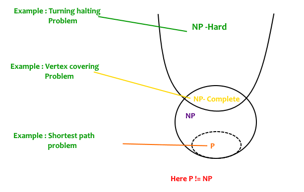
What are NP, P, NP-complete and NP-Hard problems?
P is set of problems that can be solved by a deterministic Turing machine in Polynomial time.
NP is set of decision problems that can be solved by a Non-deterministic Turing Machine in Polynomial time. P is subset of NP (any problem that can be solved by deterministic machine in polynomial time can also be solved by non-deterministic machine in polynomial time).
Informally, NP is set of decision problems which can be solved by a polynomial time via a “Lucky Algorithm”, a magical algorithm that always makes a right guess among the given set of choices (Source Ref 1).
NP-complete problems are the hardest problems in NP set. A decision problem L is NP-complete if:
1) L is in NP (Any given solution for NP-complete problems can be verified quickly, but there is no efficient known solution).
2) Every problem in NP is reducible to L in polynomial time (Reduction is defined below).
A problem is NP-Hard if it follows property 2 mentioned above, doesn’t need to follow property 1. Therefore, NP-Complete set is also a subset of NP-Hard set.
Decision vs Optimization Problems
NP-completeness applies to the realm of decision problems. It was set up this way because it’s easier to compare the difficulty of decision problems than that of optimization problems. In reality, though, being able to solve a decision problem in polynomial time will often permit us to solve the corresponding optimization problem in polynomial time (using a polynomial number of calls to the decision problem). So, discussing the difficulty of decision problems is often really equivalent to discussing the difficulty of optimization problems. (Source Ref 2).
For example, consider the vertex cover problem (Given a graph, find out the minimum sized vertex set that covers all edges). It is an optimization problem. Corresponding decision problem is, given undirected graph G and k, is there a vertex cover of size k?
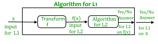
What is Reduction?
Let L1 and L2 be two decision problems. Suppose algorithm A2 solves L2. That is, if y is an input for L2 then algorithm A2 will answer Yes or No depending upon whether y belongs to L2 or not.
The idea is to find a transformation from L1 to L2 so that the algorithm A2 can be part of an algorithm A1 to solve L1.
Learning reduction in general is very important. For example, if we have library functions to solve certain problem and if we can reduce a new problem to one of the solved problems, we save a lot of time. Consider the example of a problem where we have to find minimum product path in a given directed graph where product of path is multiplication of weights of edges along the path. If we have code for Dijkstra’s algorithm to find shortest path, we can take log of all weights and use Dijkstra’s algorithm to find the minimum product path rather than writing a fresh code for this new problem.
How to prove that a given problem is NP complete?
From the definition of NP-complete, it appears impossible to prove that a problem L is NP-Complete. By definition, it requires us to that show every problem in NP is polynomial time reducible to L. Fortunately, there is an alternate way to prove it. The idea is to take a known NP-Complete problem and reduce it to L. If polynomial time reduction is possible, we can prove that L is NP-Complete by transitivity of reduction (If a NP-Complete problem is reducible to L in polynomial time, then all problems are reducible to L in polynomial time).
What was the first problem proved as NP-Complete?
There must be some first NP-Complete problem proved by definition of NP-Complete problems. SAT (Boolean satisfiability problem) is the first NP-Complete problem proved by Cook (See CLRS book for proof).
It is always useful to know about NP-Completeness even for engineers. Suppose you are asked to write an efficient algorithm to solve an extremely important problem for your company. After a lot of thinking, you can only come up exponential time approach which is impractical. If you don’t know about NP-Completeness, you can only say that I could not come with an efficient algorithm. If you know about NP-Completeness and prove that the problem as NP-complete, you can proudly say that the polynomial time solution is unlikely to exist. If there is a polynomial time solution possible, then that solution solves a big problem of computer science many scientists have been trying for years.
We will soon be discussing more NP-Complete problems and their proof for NP-Completeness.
Pseudo-polynomial Algorithms
Pseudo-polynomial Algorithms
What is Pseudo-polynomial?
An algorithm whose worst-case time complexity depends on numeric value of input (not number of inputs) is called Pseudo-polynomial algorithm.
For example, consider the problem of counting frequencies of all elements in an array of positive numbers. A pseudo-polynomial time solution for this is to first find the maximum value, then iterate from 1 to maximum value and for each value, find its frequency in array. This solution requires time according to maximum value in input array, therefore pseudo-polynomial. On the other hand, an algorithm whose time complexity is only based on number of elements in array (not value) is considered as polynomial time algorithm.
Pseudo-polynomial and NP-Completeness
Some NP-Complete problems have Pseudo Polynomial time solutions. For example, Dynamic Programming Solutions of 0-1 Knapsack, Subset-Sum and Partition problems are Pseudo-Polynomial. NP complete problems that can be solved using a pseudo-polynomial time algorithms are called weakly NP-complete.
Reference:
https://en.wikipedia.org/wiki/Pseudo-polynomial_time
Space Complexity
Space Complexity
The term Space Complexity is misused for Auxiliary Space at many places. Following are the correct definitions of Auxiliary Space and Space Complexity.
Auxiliary Space is the extra space or temporary space used by an algorithm.
Space Complexity of an algorithm is total space taken by the algorithm with respect to the input size. Space complexity includes both Auxiliary space and space used by input.
For example, if we want to compare standard sorting algorithms on the basis of space, then Auxiliary Space would be a better criteria than Space Complexity. Merge Sort uses O(n) auxiliary space, Insertion sort and Heap Sort use O(1) auxiliary space. Space complexity of all these sorting algorithms is O(n) though.
Please write comments if you find anything incorrect, or you want to share more information about the topic discussed above.
Amortized Analysis Introduction
Amortized Analysis Introduction
Amortized Analysis is used for algorithms where an occasional operation is very slow, but most of the other operations are faster. In Amortized Analysis, we analyze a sequence of operations and guarantee a worst case average time which is lower than the worst case time of a particular expensive operation.
The example data structures whose operations are analyzed using Amortized Analysis are Hash Tables, Disjoint Sets and Splay Trees.
Let us consider an example of a simple hash table insertions. How do we decide table size? There is a trade-off between space and time, if we make hash-table size big, search time becomes fast, but space required becomes high.
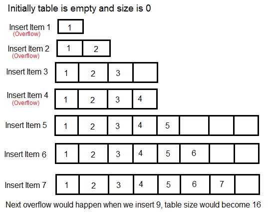
The solution to this trade-off problem is to use Dynamic Table (or Arrays). The idea is to increase size of table whenever it becomes full. Following are the steps to follow when table becomes full.
1) Allocate memory for a larger table of size, typically twice the old table.
2) Copy the contents of old table to new table.
3) Free the old table.
If the table has space available, we simply insert new item in available space.
What is the time complexity of n insertions using the above scheme?
If we use simple analysis, the worst case cost of an insertion is O(n). Therefore, worst case cost of n inserts is n * O(n) which is O(n2). This analysis gives an upper bound, but not a tight upper bound for n insertions as all insertions don’t take Θ(n) time.
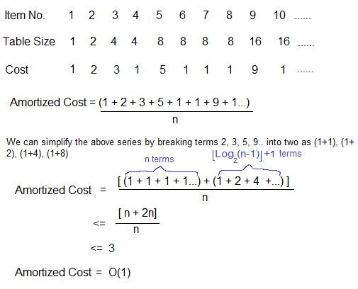
So using Amortized Analysis, we could prove that the Dynamic Table scheme has O(1) insertion time which is a great result used in hashing. Also, the concept of dynamic table is used in vectors in C++, ArrayList in Java.
Following are few important notes.
1) Amortized cost of a sequence of operations can be seen as expenses of a salaried person. The average monthly expense of the person is less than or equal to the salary, but the person can spend more money in a particular month by buying a car or something. In other months, he or she saves money for the expensive month.
2) The above Amortized Analysis done for Dynamic Array example is called Aggregate Method. There are two more powerful ways to do Amortized analysis called Accounting Method and Potential Method. We will be discussing the other two methods in separate posts.
3) The amortized analysis doesn’t involve probability. There is also another different notion of average case running time where algorithms use randomization to make them faster and expected running time is faster than the worst case running time. These algorithms are analyzed using Randomized Analysis. Examples of these algorithms are Randomized Quick Sort, Quick Select and Hashing. We will soon be covering Randomized analysis in a different post.
Solving Recurrences
Solving Recurrences
In the previous post, we discussed analysis of loops. Many algorithms are recursive in nature. When we analyze them, we get a recurrence relation for time complexity. We get running time on an input of size n as a function of n and the running time on inputs of smaller sizes. For example in Merge Sort, to sort a given array, we divide it in two halves and recursively repeat the process for the two halves. Finally we merge the results. Time complexity of Merge Sort can be written as T(n) = 2T(n/2) + cn. There are many other algorithms like Binary Search, Tower of Hanoi, etc.
There are mainly three ways for solving recurrences.
1) Substitution Method: We make a guess for the solution and then we use mathematical induction to prove the the guess is correct or incorrect.
For example consider the recurrence T(n) = 2T(n/2) + n

We guess the solution as T(n) = O(nLogn). Now we use induction
to prove our guess.

We need to prove that T(n) <= cnLogn. We can assume that it is true
for values smaller than n.

T(n) = 2T(n/2) + n
    <= cn/2Log(n/2) + n
    =  cnLogn - cnLog2 + n
    =  cnLogn - cn + n
    <= cnLogn
2) Recurrence Tree Method: In this method, we draw a recurrence tree and calculate the time taken by every level of tree. Finally, we sum the work done at all levels. To draw the recurrence tree, we start from the given recurrence and keep drawing till we find a pattern among levels. The pattern is typically a arithmetic or geometric series.
For example consider the recurrence relation
T(n) = T(n/4) + T(n/2) + cn2

           cn2
         /      \
     T(n/4)     T(n/2)

If we further break down the expression T(n/4) and T(n/2),
we get following recursion tree.

                cn2
           /           \
       c(n2)/16      c(n2)/4
      /      \          /     \
  T(n/16)     T(n/8)  T(n/8)    T(n/4)
Breaking down further gives us following
                 cn2
            /            \
       c(n2)/16          c(n2)/4
       /      \            /      \
c(n2)/256   c(n2)/64  c(n2)/64    c(n2)/16
 /    \      /    \    /    \       /    \

To know the value of T(n), we need to calculate sum of tree
nodes level by level. If we sum the above tree level by level,
we get the following series
T(n)  = c(n^2 + 5(n^2)/16 + 25(n^2)/256) + ....
The above series is geometrical progression with ratio 5/16.

To get an upper bound, we can sum the infinite series.
We get the sum as (n2)/(1 - 5/16) which is O(n2)
3) Master Method:
Master Method is a direct way to get the solution. The master method works only for following type of recurrences or for recurrences that can be transformed to following type.
T(n) = aT(n/b) + f(n) where a >= 1 and b > 1
There are following three cases:
1. If f(n) = Θ(nc) where c < Logba then T(n) = Θ(nLogba)
2. If f(n) = Θ(nc) where c = Logba then T(n) = Θ(ncLog n)
3.If f(n) = Θ(nc) where c > Logba then T(n) = Θ(f(n))
How does this work?
Master method is mainly derived from recurrence tree method. If we draw recurrence tree of T(n) = aT(n/b) + f(n), we can see that the work done at root is f(n) and work done at all leaves is Θ(nc) where c is Logba. And the height of recurrence tree is Logbn

In recurrence tree method, we calculate total work done. If the work done at leaves is polynomially more, then leaves are the dominant part, and our result becomes the work done at leaves (Case 1). If work done at leaves and root is asymptotically same, then our result becomes height multiplied by work done at any level (Case 2). If work done at root is asymptotically more, then our result becomes work done at root (Case 3).
Examples of some standard algorithms whose time complexity can be evaluated using Master Method
Merge Sort: T(n) = 2T(n/2) + Θ(n). It falls in case 2 as c is 1 and Logba] is also 1. So the solution is Θ(n Logn)
Binary Search: T(n) = T(n/2) + Θ(1). It also falls in case 2 as c is 0 and Logba is also 0. So the solution is Θ(Logn)
Notes:
1) It is not necessary that a recurrence of the form T(n) = aT(n/b) + f(n) can be solved using Master Theorem. The given three cases have some gaps between them. For example, the recurrence T(n) = 2T(n/2) + n/Logn cannot be solved using master method.
2) Case 2 can be extended for f(n) = Θ(ncLogkn)
If f(n) = Θ(ncLogkn) for some constant k >= 0 and c = Logba, then T(n) = Θ(ncLogk+1n)
Analysis of Loops
Analysis of Loops
We have discussed Asymptotic Analysis, Worst, Average and Best Cases and Asymptotic Notations in previous posts. In this post, analysis of iterative programs with simple examples is discussed.
1) O(1): Time complexity of a function (or set of statements) is considered as O(1) if it doesn’t contain loop, recursion and call to any other non-constant time function.
// set of non-recursive and non-loop statements
For example swap() function has O(1) time complexity.
A loop or recursion that runs a constant number of times is also considered as O(1). For example the following loop is O(1).
   // Here c is a constant
   for (int i = 1; i <= c; i++) {
        // some O(1) expressions
   }
2) O(n): Time Complexity of a loop is considered as O(n) if the loop variables is incremented / decremented by a constant amount. For example following functions have O(n) time complexity.
   // Here c is a positive integer constant
   for (int i = 1; i <= n; i += c) {
        // some O(1) expressions
   }

   for (int i = n; i > 0; i -= c) {
        // some O(1) expressions
   }
3) O(nc): Time complexity of nested loops is equal to the number of times the innermost statement is executed. For example the following sample loops have O(n2) time complexity
   for (int i = 1; i <=n; i += c) {
       for (int j = 1; j <=n; j += c) {
          // some O(1) expressions
       }
   }

   for (int i = n; i > 0; i -= c) {
       for (int j = i+1; j <=n; j += c) {
          // some O(1) expressions
   }
For example Selection sort and Insertion Sort have O(n2) time complexity.
4) O(Logn) Time Complexity of a loop is considered as O(Logn) if the loop variables is divided / multiplied by a constant amount.
   for (int i = 1; i <=n; i *= c) {
       // some O(1) expressions
   }
   for (int i = n; i > 0; i /= c) {
       // some O(1) expressions
   }
For example Binary Search(refer iterative implementation) has O(Logn) time complexity. Let us see mathematically how it is O(Log n). The series that we get in first loop is 1, c, c2, c3, … ck. If we put k equals to Logcn, we get cLogcnwhich is n.
5) O(LogLogn) Time Complexity of a loop is considered as O(LogLogn) if the loop variables is reduced / increased exponentially by a constant amount.
   // Here c is a constant greater than 1
   for (int i = 2; i <=n; i = pow(i, c)) {
       // some O(1) expressions
   }
   //Here fun is sqrt or cuberoot or any other constant root
   for (int i = n; i > 0; i = fun(i)) {
       // some O(1) expressions
   }
See this for mathematical details.
How to combine time complexities of consecutive loops?
When there are consecutive loops, we calculate time complexity as sum of time complexities of individual loops.
   for (int i = 1; i <=m; i += c) {
        // some O(1) expressions
   }
   for (int i = 1; i <=n; i += c) {
        // some O(1) expressions
   }
   Time complexity of above code is O(m) + O(n) which is O(m+n)
   If m == n, the time complexity becomes O(2n) which is O(n).
How to calculate time complexity when there are many if, else statements inside loops?
As discussed here, worst case time complexity is the most useful among best, average and worst. Therefore we need to consider worst case. We evaluate the situation when values in if-else conditions cause maximum number of statements to be executed.
For example consider the linear search function where we consider the case when element is present at the end or not present at all.
When the code is too complex to consider all if-else cases, we can get an upper bound by ignoring if else and other complex control statements.
How to calculate time complexity of recursive functions?
Time complexity of a recursive function can be written as a mathematical recurrence relation. To calculate time complexity, we must know how to solve recurrences. We will soon be discussing recurrence solving techniques as a separate post.