The model of a parallel algorithm is developed by considering a strategy for dividing the data and processing method and applying a suitable strategy to reduce interactions. In this chapter, we will discuss the following Parallel Algorithm Models −

• Data parallel model
• Task graph model
• Work pool model
• Master slave model
• Producer consumer or pipeline model
• Hybrid model

Data Parallel

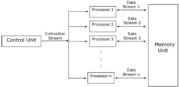
In data parallel model, tasks are assigned to processes and each task performs similar types of operations on different data. Data parallelism is a consequence of single operations that is being applied on multiple data items.

Data-parallel model can be applied on shared-address spaces and message-passing paradigms. In data-parallel model, interaction overheads can be reduced by selecting a locality preserving decomposition, by using optimized collective interaction routines, or by overlapping computation and interaction.

The primary characteristic of data-parallel model problems is that the intensity of data parallelism increases with the size of the problem, which in turn makes it possible to use more processes to solve larger problems.

Example − Dense matrix multiplication.

Task Graph Model

In the task graph model, parallelism is expressed by a task graph. A task graph can be either trivial or nontrivial. In this model, the correlation among the tasks are utilized to promote locality or to minimize interaction costs. This model is enforced to solve problems in which the quantity of data associated with the tasks is huge compared to the number of computation associated with them. The tasks are assigned to help improve the cost of data movement among the tasks.

Examples − Parallel quick sort, sparse matrix factorization, and parallel algorithms derived via divide-and-conquer approach.

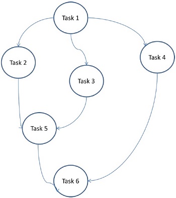
Here, problems are divided into atomic tasks and implemented as a graph. Each task is an independent unit of job that has dependencies on one or more antecedent task. After the completion of a task, the output of an antecedent task is passed to the dependent task. A task with antecedent task starts execution only when its entire antecedent task is completed. The final output of the graph is received when the last dependent task is completed (Task 6 in the above figure).

Work Pool Model

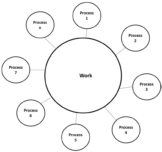
In work pool model, tasks are dynamically assigned to the processes for balancing the load. Therefore, any process may potentially execute any task. This model is used when the quantity of data associated with tasks is comparatively smaller than the computation associated with the tasks.

There is no desired pre-assigning of tasks onto the processes. Assigning of tasks is centralized or decentralized. Pointers to the tasks are saved in a physically shared list, in a priority queue, or in a hash table or tree, or they could be saved in a physically distributed data structure.

The task may be available in the beginning, or may be generated dynamically. If the task is generated dynamically and a decentralized assigning of task is done, then a termination detection algorithm is required so that all the processes can actually detect the completion of the entire program and stop looking for more tasks.

Example − Parallel tree search

Master-Slave Model

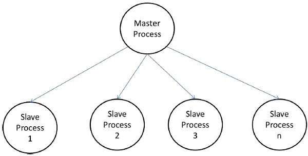
In the master-slave model, one or more master processes generate task and allocate it to slave processes. The tasks may be allocated beforehand if −

• the master can estimate the volume of the tasks, or
• a random assigning can do a satisfactory job of balancing load, or
• slaves are assigned smaller pieces of task at different times.

This model is generally equally suitable to shared-address-space or message-passing paradigms, since the interaction is naturally two ways.

In some cases, a task may need to be completed in phases, and the task in each phase must be completed before the task in the next phases can be generated. The master-slave model can be generalized to hierarchical or multi-level master-slave model in which the top level master feeds the large portion of tasks to the second-level master, who further subdivides the tasks among its own slaves and may perform a part of the task itself.

Precautions in using the master-slave model

Care should be taken to assure that the master does not become a congestion point. It may happen if the tasks are too small or the workers are comparatively fast.

The tasks should be selected in a way that the cost of performing a task dominates the cost of communication and the cost of synchronization.

Asynchronous interaction may help overlap interaction and the computation associated with work generation by the master.

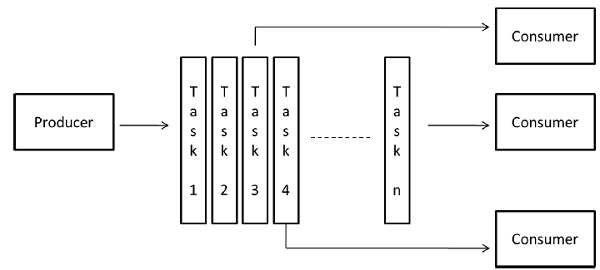
Pipeline Model

It is also known as the producer-consumer model. Here a set of data is passed on through a series of processes, each of which performs some task on it. Here, the arrival of new data generates the execution of a new task by a process in the queue. The processes could form a queue in the shape of linear or multidimensional arrays, trees, or general graphs with or without cycles.

This model is a chain of producers and consumers. Each process in the queue can be considered as a consumer of a sequence of data items for the process preceding it in the queue and as a producer of data for the process following it in the queue. The queue does not need to be a linear chain; it can be a directed graph. The most common interaction minimization technique applicable to this model is overlapping interaction with computation.

Example − Parallel LU factorization algorithm.

Hybrid Models

A hybrid algorithm model is required when more than one model may be needed to solve a problem.

A hybrid model may be composed of either multiple models applied hierarchically or multiple models applied sequentially to different phases of a parallel algorithm.

Example − Parallel quick sort