

Hashing
Suppose we want to design a system for storing employee records keyed using phone numbers. And we want following queries to be performed efficiently:
- Insert a phone number and corresponding information.
- Search a phone number and fetch the information.
- Delete a phone number and related information.
We can think of using the following data structures to maintain information about different phone numbers.
- Array of phone numbers and records.
- Linked List of phone numbers and records.
- Balanced binary search tree with phone numbers as keys.
- Direct Access Table.
For arrays and linked lists, we need to search in a linear fashion, which can be costly in practice. If we use arrays and keep the data sorted, then a phone number can be searched in O(Logn) time using Binary Search, but insert and delete operations become costly as we have to maintain sorted order.
With balanced binary search tree, we get moderate search, insert and delete times. All of these operations can be guaranteed to be in O(Logn) time.
Another solution that one can think of is to use a direct access table where we make a big array and use phone numbers as index in the array. An entry in array is NIL if phone number is not present, else the array entry stores pointer to records corresponding to phone number. Time complexity wise this solution is the best among all, we can do all operations in O(1) time. For example to insert a phone number, we create a record with details of given phone number, use phone number as index and store the pointer to the created record in table.
This solution has many practical limitations. First problem with this solution is extra space required is huge. For example if phone number is n digits, we need O(m * 10n) space for table where m is size of a pointer to record. Another problem is an integer in a programming language may not store n digits.
Due to above limitations, Direct Access Table cannot always be used. Hashing is the solution that can be used in almost all such situations and performs extremely well compared to above data structures like Array, Linked List, Balanced BST in practice. With hashing we get O(1) search time on average (under reasonable assumptions) and O(n) in worst case.
Hashing is an improvement over Direct Access Table. The idea is to use hash function that converts a given phone number or any other key to a smaller number and uses the small number as index in a table called hash table.
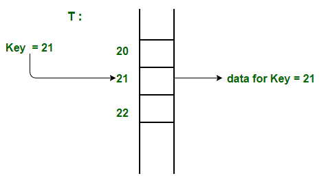
Hash Function:
A function that converts a given big phone number to a small practical integer value. The mapped integer value is used as an index in hash table. In simple terms, a hash function maps a big number or string to a small integer that can be used as index in hash table.
A good hash function should have following properties
1) Efficiently computable.
2) Should uniformly distribute the keys (Each table position equally likely for each key)
For example for phone numbers a bad hash function is to take first three digits. A better function is consider last three digits. Please note that this may not be the best hash function. There may be better ways.
Hash Table:
An array that stores pointers to records corresponding to a given phone number. An entry in hash table is NIL if no existing phone number has hash function value equal to the index for the entry.
Index Mapping (or Trivial Hashing) with negatives allowed
Given a limited range array contains both positive and non positive numbers, i.e., elements are in range from -MAX to +MAX. Our task is to search if some number is present in the array or not in O(1) time.
Since range is limited, we can use index mapping (or trivial hashing). We use values as index in a big array. Therefore we can search and insert elements in O(1) time.
How to handle negative numbers?
The idea is to use a 2D array of size hash[MAX+1][2]
Algorithm:
Assign all the values of the hash matrix as 0.
Traverse the given array:
    If the element ele is non negative assign
        hash[ele][0] as 1.
    Else take the absolute value of ele and
         assign hash[ele][1] as 1.
To search any element x in the array.
- If X is non-negative check if hash[X][0] is 1 or not. If hash[X][0] is one then the number is present else not present.
- If X is negative take absolute vale of X and then check if hash[X][1] is 1 or not. If hash[X][1] is one then the number is present
What is Collision?
Since a hash function gets us a small number for a key which is a big integer or string, there is possibility that two keys result in same value. The situation where a newly inserted key maps to an already occupied slot in hash table is called collision and must be handled using some collision handling technique.
What are the chances of collisions with large table?
Collisions are very likely even if we have big table to store keys. An important observation is Birthday Paradox. With only 23 persons, the probability that two people have same birthday is 50%.
How to handle Collisions?
There are mainly two methods to handle collision:
1) Separate Chaining
2) Open Addressing
In this article, only separate chaining is discussed. We will be discussing Open addressing in next post.
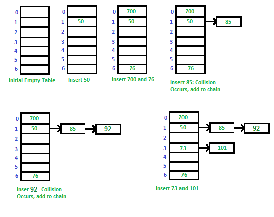
Separate Chaining:
The idea is to make each cell of hash table point to a linked list of records that have same hash function value.
Let us consider a simple hash function as “key mod 7” and sequence of keys as 50, 700, 76, 85, 92, 73, 101.
C++ program for hashing with chaining
Advantages:
1) Simple to implement.
2) Hash table never fills up, we can always add more elements to chain.
3) Less sensitive to the hash function or load factors.
4) It is mostly used when it is unknown how many and how frequently keys may be inserted or deleted.
Disadvantages:
1) Cache performance of chaining is not good as keys are stored using linked list. Open addressing provides better cache performance as everything is stored in same table.
2) Wastage of Space (Some Parts of hash table are never used)
3) If the chain becomes long, then search time can become O(n) in worst case.
4) Uses extra space for links.
Performance of Chaining:
Performance of hashing can be evaluated under the assumption that each key is equally likely to be hashed to any slot of table (simple uniform hashing).
 m = Number of slots in hash table
 n = Number of keys to be inserted in hash table

 Load factor α = n/m

 Expected time to search = O(1 + α)

 Expected time to insert/delete = O(1 + α)

 Time complexity of search insert and delete is
 O(1) if  α is O(1)
Open Addressing
Like separate chaining, open addressing is a method for handling collisions. In Open Addressing, all elements are stored in the hash table itself. So at any point, size of the table must be greater than or equal to the total number of keys (Note that we can increase table size by copying old data if needed).
Insert(k): Keep probing until an empty slot is found. Once an empty slot is found, insert k.
Search(k): Keep probing until slot’s key doesn’t become equal to k or an empty slot is reached.
Delete(k): Delete operation is interesting. If we simply delete a key, then search may fail. So slots of deleted keys are marked specially as “deleted”.
Insert can insert an item in a deleted slot, but the search doesn’t stop at a deleted slot.
Open Addressing is done following ways:
a) Linear Probing: In linear probing, we linearly probe for next slot. For example, typical gap between two probes is 1 as taken in below example also.
let hash(x) be the slot index computed using hash function and S be the table size
If slot hash(x) % S is full, then we try (hash(x) + 1) % S
If (hash(x) + 1) % S is also full, then we try (hash(x) + 2) % S
If (hash(x) + 2) % S is also full, then we try (hash(x) + 3) % S
..................................................
..................................................
Let us consider a simple hash function as “key mod 7” and sequence of keys as 50, 700, 76, 85, 92, 73, 101.
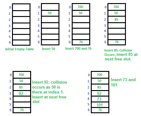
Clustering: The main problem with linear probing is clustering, many consecutive elements form groups and it starts taking time to find a free slot or to search an element.
b) Quadratic Probing We look for i2‘th slot in i’th iteration.
let hash(x) be the slot index computed using hash function.
If slot hash(x) % S is full, then we try (hash(x) + 1*1) % S
If (hash(x) + 1*1) % S is also full, then we try (hash(x) + 2*2) % S
If (hash(x) + 2*2) % S is also full, then we try (hash(x) + 3*3) % S
..................................................
..................................................
c) Double Hashing We use another hash function hash2(x) and look for i*hash2(x) slot in i’th rotation.
let hash(x) be the slot index computed using hash function.
If slot hash(x) % S is full, then we try (hash(x) + 1*hash2(x)) % S
If (hash(x) + 1*hash2(x)) % S is also full, then we try (hash(x) + 2*hash2(x)) % S
If (hash(x) + 2*hash2(x)) % S is also full, then we try (hash(x) + 3*hash2(x)) % S
..................................................
..................................................
See this for step by step diagrams.
Comparison of above three:
Linear probing has the best cache performance but suffers from clustering. One more advantage of Linear probing is easy to compute.
Quadratic probing lies between the two in terms of cache performance and clustering.
Double hashing has poor cache performance but no clustering. Double hashing requires more computation time as two hash functions need to be computed.
| S.No. | Separate Chaining | Open Addressing |
| 1. | Chaining is Simpler to implement. | Open Addressing requires more computation. |
| 2. | In chaining, Hash table never fills up, we can always add more elements to chain. | In open addressing, table may become full. |
| 3. | Chaining is Less sensitive to the hash function or load factors. | Open addressing requires extra care for to avoid clustering and load factor. |
| 4. | Chaining is mostly used when it is unknown how many and how frequently keys may be inserted or deleted. | Open addressing is used when the frequency and number of keys is known. |
| 5. | Cache performance of chaining is not good as keys are stored using linked list. | Open addressing provides better cache performance as everything is stored in the same table. |
| 6. | Wastage of Space (Some Parts of hash table in chaining are never used). | In Open addressing, a slot can be used even if an input doesn’t map to it. |
| 7. | Chaining uses extra space for links. | No links in Open addressing |
Performance of Open Addressing:
Like Chaining, the performance of hashing can be evaluated under the assumption that each key is equally likely to be hashed to any slot of the table (simple uniform hashing)
 m = Number of slots in the hash table
 n = Number of keys to be inserted in the hash table

 Load factor α = n/m  ( < 1 )

 Expected time to search/insert/delete < 1/(1 - α)

 So Search, Insert and Delete take (1/(1 - α)) time
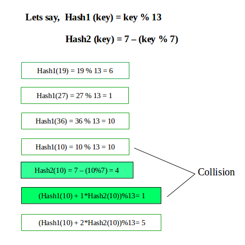
Double Hashing
Double hashing is a collision resolving technique in Open Addressed Hash tables. Double hashing uses the idea of applying a second hash function to key when a collision occurs.
(hash1(key) + i * hash2(key)) % TABLE_SIZE
Here hash1() and hash2() are hash functions and TABLE_SIZE
is size of hash table.
(We repeat by increasing i when collision occurs)
First hash function is typically hash1(key) = key % TABLE_SIZE
A popular second hash function is : hash2(key) = PRIME – (key % PRIME) where PRIME is a prime smaller than the TABLE_SIZE.
A good second Hash function is:
- It must never evaluate to zero
- Must make sure that all cells can be probed
C++ program for Double Hashing