

Secondary Storage Structure
Secondary storage devices are those devices whose memory is non volatile, meaning, the stored data will be intact even if the system is turned off. Here are a few things worth noting about secondary storage.
- Secondary storage is also called auxiliary storage.
- Secondary storage is less expensive when compared to primary memory like RAMs.
- The speed of the secondary storage is also lesser than that of primary storage.
- Hence, the data which is less frequently accessed is kept in the secondary storage.
- A few examples are magnetic disks, magnetic tapes, removable thumb drives etc.
Magnetic Disk Structure
In modern computers, most of the secondary storage is in the form of magnetic disks. Hence, knowing the structure of a magnetic disk is necessary to understand how the data in the disk is accessed by the computer.
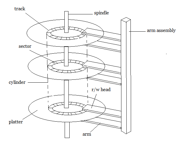
Structure of a magnetic disk
A magnetic disk contains several platters. Each platter is divided into circular shaped tracks. The length of the tracks near the centre is less than the length of the tracks farther from the centre. Each track is further divided into sectors, as shown in the figure.
Tracks of the same distance from centre form a cylinder. A read-write head is used to read data from a sector of the magnetic disk.
The speed of the disk is measured as two parts:
- Transfer rate: This is the rate at which the data moves from disk to the computer.
- Random access time: It is the sum of the seek time and rotational latency.
Seek time is the time taken by the arm to move to the required track. Rotational latency is defined as the time taken by the arm to reach the required sector in the track.
Even though the disk is arranged as sectors and tracks physically, the data is logically arranged and addressed as an array of blocks of fixed size. The size of a block can be 512 or 1024 bytes. Each logical block is mapped with a sector on the disk, sequentially. In this way, each sector in the disk will have a logical address.
Disk Scheduling Algorithms
On a typical multiprogramming system, there will usually be multiple disk access requests at any point of time. So those requests must be scheduled to achieve good efficiency. Disk scheduling is similar to process scheduling. Some of the disk scheduling algorithms are described below.
First Come First Serve:
This algorithm performs requests in the same order asked by the system. Let’s take an example where the queue has the following requests with cylinder numbers as follows:
98, 183, 37, 122, 14, 124, 65, 67
Assume the head is initially at cylinder 56. The head moves in the given order in the queue i.e., 56->98->183->….->67.
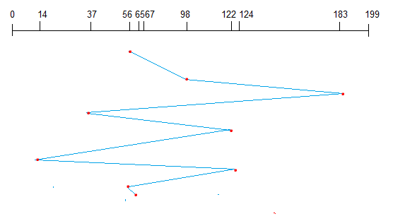
FCFS Disk Scheduling
Shortest Seek Time First (SSTF):
Here the position which is closest to the current head position is chosen first. Consider the previous example where disk queue looks like,
98, 183, 37, 122, 14, 124, 65, 67
Assume the head is initially at cylinder 56. The next closest cylinder to 56 is 65, and then the next nearest one is 67, then 37, 14, so on.
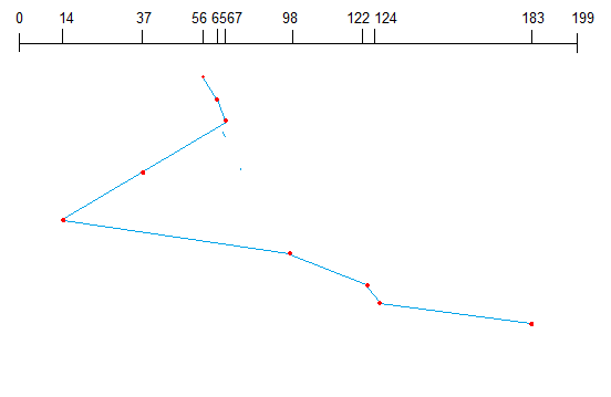
SSTF Disk Scheduling
SCAN algorithm:
This algorithm is also called the elevator algorithm because of it’s behavior. Here, first the head moves in a direction (say backward) and covers all the requests in the path. Then it moves in the opposite direction and covers the remaining requests in the path. This behavior is similar to that of an elevator. Let’s take the previous example,
98, 183, 37, 122, 14, 124, 65, 67
Assume the head is initially at cylinder 56. The head moves in backward direction and accesses 37 and 14. Then it goes in the opposite direction and accesses the cylinders as they come in the path.
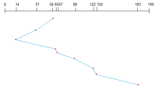
SCAN algorithm